
In the last two blog posts (EI 1 and EI 2), we have looked at the basics of investments and cash flows from capital investment. In this post, we will look at cash flows from ECM’s and avoided costs in general.
Before getting to cash flows of an ECM, another general, MBA case study version should help shed light on the nature of avoided costs. A company is in the business of selling widgets and they are considering buying a $10 million machine that will lower their variable costs by $5 a widget. The company sold a million widgets last year. The obvious answer is that the machine will save 5 million dollars, but this answer would be wrong. The actual cash flows depend on how many widgets are produced.
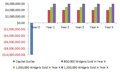
The actual cash flows from the device are equal to (the number of widgets produced)*($5.00). Instead of having cash flows set in stone when the machine is bought, the machine will have a higher return if sales happen to be higher and a lower return if sales are lower. To put it in more precise terms, the savings of the machine are the difference of the actual costs and the costs in a world where the machine did not exist.
External Factors and ECM Payback
The clearest parallel between ECM’s and the widget machine is the nature of energy costs. Instead of saving $5 a widget, ECM’s save energy without any regard to the price of that energy. The project directly save kWh, therms, gallons of water and other energy units, and only save money through how much those units cost on the bill. So if a site currently has a rate of $0.12/kWh and an ECM will save 100,000 kWh a year, the savings will not necessarily be $12,000. The savings will go up as energy costs go up and savings will go down as energy costs will go down.
Less clear is the parallel between the number of widgets variable above and energy variables other than rate, such as weather, occupancy and changes in usage patterns. An energy manager instinctually knows that a hotter summer means a new HVAC unit will not save as much as expected. But how does one go about quantifying that in a relatively simple, straightforward way?
Remember how we calculated the savings for the widget machine. The widget machine’s savings are the actual costs versus the costs of a world where the widget machine does not exist. Similarly, an ECM’s energy savings are the difference of the actual energy usage and the energy usage in a world where the ECM never happened. Note that this definition says energy, not costs. The cost savings are simply multiplying the energy savings times the rate. The technical name for “energy usage in a world where the ECM never happened” is a baseline.
Without getting into all the details and nuances of possible baselines, here is a relatively simple example. A new set of HVAC units is put into service in March this year. A simple year-over-year graph of the electrical usage is shown below, with clear savings from 2011 to 2012. By the way, these numbers were made up on the spot and are not any real-world data.
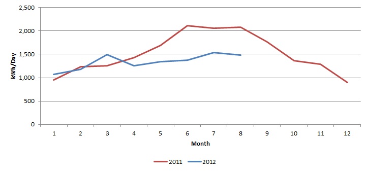
At first glance, one may want to just take the difference between the 2012 and 2011 usage, multiply that by the 2012 rate, and call that the savings. In many ad hoc analyses, this method is quite popular and I do it quite a bit myself to show general trends. A true analysis however needs to create a baseline showing usage if the ECM never happened.
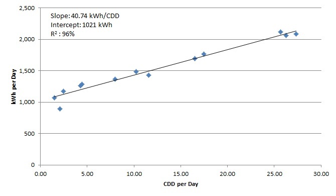
The baseline is a regression model where some inputs, like weather or occupancy, are fitted to the actual outputs. In this simple example, the only input will be the cooling load on the building. While a measure like the month’s average temperature could be used, cooling degree days have much better predictive ability. For a good summary of cooling degree days, go here.
It is also important which of the months one picks to generate the model. It is crucial that the months during or after the ECM implementation is not used. Unless the ECM changed nothing at the site, the months after will respond differently to cooling degree days and other variables versus the months before. One should also not go too far back, such as 24 months, since the site characteristics may have changed over that time period. For this example, I will go back 12 months.
A simple regression trendline of the 12 months before is shown below. On relatively simple sites such as retail, the R2 can often be over 90%. Notice that the independent and dependent variables are CDD/day and Usage/day respectively. Using per-day numbers corrects for how one would expect March to have higher usage than February just from having 31 days instead of 28.
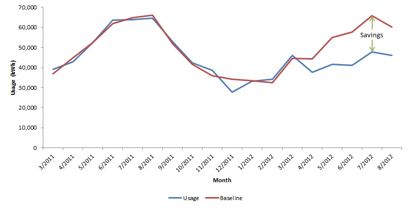
The graph below is the final analysis to give true savings. Instead of showing year-over-year usages, the two lines are the actual usage and the baseline usage. Since the baseline models the actual usage before the ECM’s, the baseline tracks closely with the actual before the ECM’s were implemented. Afterward, the baseline and the actual diverge. The baseline shows that the site would have used far more energy than it and the difference between the actual and the baseline is multiplied by the rate for that month to give the savings.
In the next and final section, we will look at how this framework can be useful for homeowners and we will sum up the blog series.